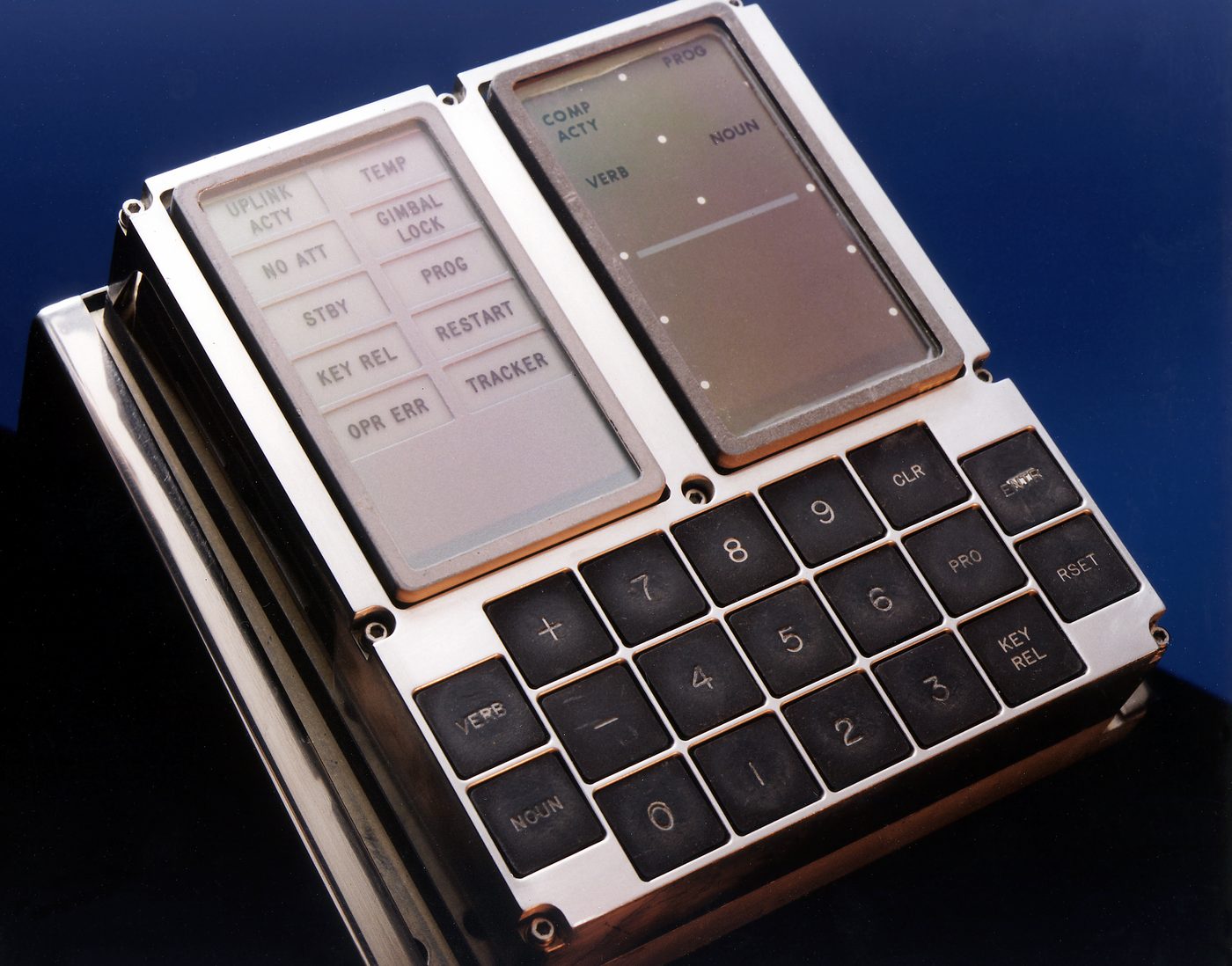
DSKY — Volume 6 — Inside the AGC: Architecture & Instruction Set

About This Volume

The previous volumes treated the Apollo Guidance Computer (AGC) from the outside: as the box behind the DSKY, the partner the astronauts spoke to in verbs and nouns. This volume opens the lid and looks at the machine itself — not as a relic to be admired, but as a working architecture with rules you can actually understand. We will follow a single number from its representation in a sixteen-bit word, through the registers that held it and the clock that drove it, into the small but cleverly extended instruction set that manipulated it, and finally up into the interpretive layer that let a tiny machine do orbital mathematics it had no native ability to perform.

The AGC was not fast, not large, and not, by the standards of its own decade, exotic in its logic. What made it remarkable was the discipline of its design — the way a severe set of constraints (weight, power, volume, reliability) was answered by an architecture in which almost nothing was wasted. Understanding that architecture is the best possible preparation for the volumes that follow, where we watch the software executive (Volume 10) schedule real work on top of these bones. Throughout, the canonical figures are the Block II machine: a sixteen-bit word, roughly 36,864 words of fixed memory and 2,048 words of erasable memory, a 2.048 MHz clock, and a basic memory cycle of about 11.7 microseconds.

The Word

Everything in the AGC begins with the word: sixteen bits. But that headline number is slightly misleading, because the bits did not all carry numerical information. One bit — the sixteenth — was a parity bit, present purely for error detection. The remaining fifteen bits were the data the machine actually computed on. So when engineers call the AGC a “fifteen-bit machine,” they are counting the useful bits and setting the housekeeping bit aside.

Parity worked by a simple, robust rule: a small generator circuit set the parity bit to whatever value (0 or 1) made the total count of 1-bits in the word odd. Every time a word was read from memory, a checking circuit recounted the ones. If the total came out even, a bit had flipped somewhere and the word was presumed corrupt. This odd-parity scheme caught any single-bit error in storage — cheap insurance for a computer that could never be sent back to the shop. Crucially, the parity bit took no part in arithmetic; the logic operated on the fifteen data bits and simply ignored bit sixteen during computation.

Numbers themselves were stored in ones’-complement representation. This is worth a moment, because it is the source of one of the AGC’s small charms. In ones’ complement, you form the negative of a number by inverting every bit — flipping each 0 to 1 and each 1 to 0. There is no separate “negate and add one” step, as in the now-universal two’s complement. The high-order bit serves as a sign: 0 for positive, 1 for negative. A signed quantity therefore lived in fourteen magnitude bits plus one sign bit, and a great many of the values the navigation software handled were exactly that — fourteen bits and a sign.

Ones’ complement has one famous quirk: it has two zeroes. “Positive zero” is all bits 0; “negative zero” is all bits 1 (the inversion of positive zero). The hardware and software had to be written to treat both as zero, and AGC programmers learned to respect the distinction — negative zero was a real bit pattern that could arise from a subtraction and had to be handled with care. The benefit that justified the quirk was symmetry and simplicity in the adder: addition and subtraction of signed numbers fell out of the same bit-inversion logic, and an end-around carry (a carry out of the top, wrapping back into the bottom) kept the arithmetic consistent.

Beyond the parity bit, the internal working format added a little more nuance. Inside the central processor a value could carry an overflow bit above the sign, letting the machine notice when a sum had grown too large for fourteen magnitude bits and react accordingly — essential when integrating equations of motion where a runaway value must be detected, not silently wrapped.

Timing: Two Megahertz and the Memory Cycle

The AGC’s heartbeat was a 2.048 MHz crystal oscillator. From this master frequency the machine derived everything else. The 2.048 MHz signal was divided by two to yield a four-phase 1.024 MHz clock, and it was at that lower rate that the processor stepped through its internal operations.

The fundamental unit of work was the memory cycle time, or MCT, lasting about 11.7 microseconds (11.72 µs to be precise). Every basic operation was measured in MCTs. Internally each MCT was subdivided into twelve short time pulses, labelled T1 through T12, each just under a microsecond long. These twelve pulses orchestrated the micro-steps of an instruction: reading a word from memory, routing it through the central registers, passing it through the adder, and writing a result back. Because core memory is destructive to read — sensing a core’s state clears it — part of every cycle was spent rewriting what had just been read, and the twelve-pulse structure made room for that rewrite automatically.

Most basic instructions consumed a small, fixed number of MCTs — typically one or two, with the multiply and divide operations taking longer. That puts the AGC’s raw throughput on the order of tens of thousands of additions per second: roughly one addition every couple of cycles, a couple of cycles every twenty-odd microseconds. By modern reckoning this is glacial; for 1966 flight hardware it was a carefully balanced figure, fast enough to close a guidance loop several times a second while sipping the few tens of watts the spacecraft could spare.

The Central Registers

The AGC had no large bank of CPU registers in the modern sense. Instead, a handful of central registers lived at the very bottom of erasable memory — addresses so low that the hardware gave them special treatment. Because they were memory locations, ordinary instructions could read and write them as easily as any other word, which kept the instruction set small. The most important ones:

Reg	Name	Role
A	Accumulator	The main working register; nearly every arithmetic op touched it
L	Lower accumulator	Held the low half of double-length products and results
Q	Return address	TC stashed the return point here, enabling subroutine calls
Z	Program counter	The address of the next instruction to execute
BB / EB / FB	Bank registers	Selected which bank of fixed or erasable memory was in view

Z deserves a note: by making the program counter an ordinary, addressable register, the designers turned “jump to an address” into nothing more exotic than “store a value into Z.” The same economy applied throughout — control flow, subroutine linkage, and indexing were all expressed as moves and stores into these privileged low locations.

Alongside the central registers sat a second special class: the counter registers. These were erasable locations that the hardware itself could increment or decrement, asynchronously, in response to external pulses. The mechanism was the counter interrupt (sometimes called an involuntary or unprogrammed sequence): when a pulse arrived — a tick of the spacecraft clock, an increment from a gyro, a count from the rendezvous radar — the hardware briefly stole a memory cycle, bumped the appropriate counter, and returned, all without the running program’s knowledge or permission. This is how the AGC kept time and tallied incoming data even as it computed. Master timekeeping registers were chained so that overflow of a low-order counter rippled into the next, building a continuously running clock that the executive could consult at any moment. The counters were, in effect, a layer of free hardware concurrency beneath the software.

The Instruction Set

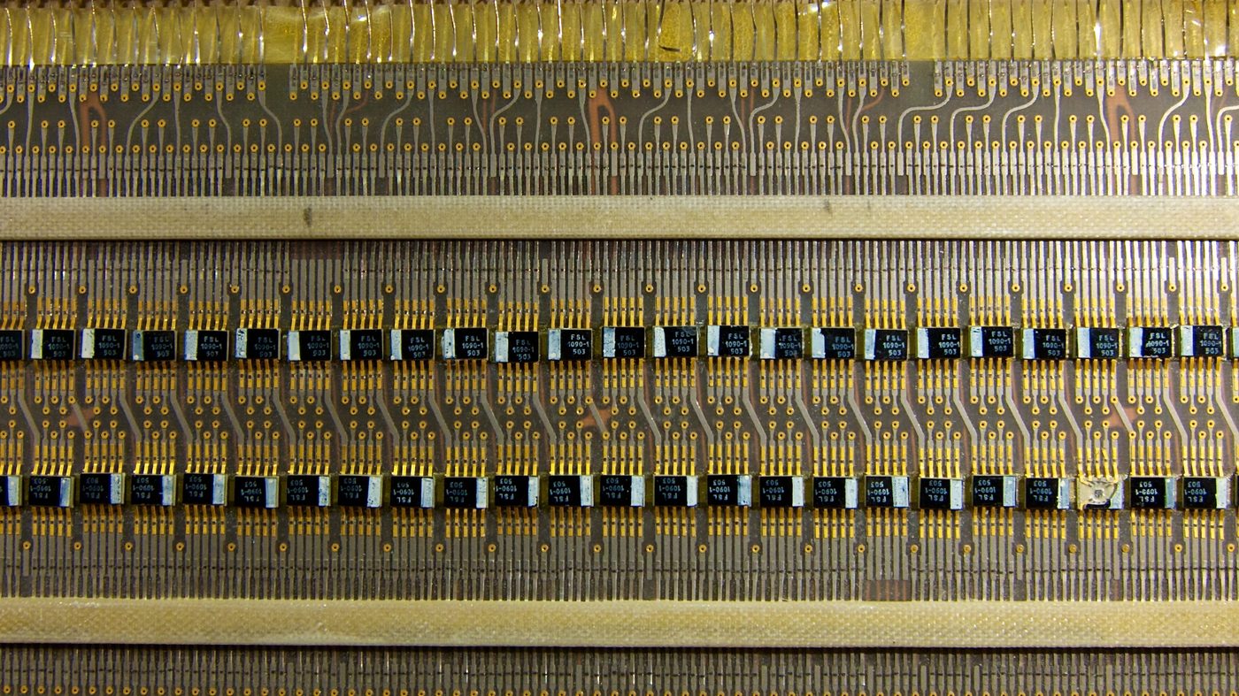
The AGC’s native instruction set was deliberately tiny, and there is a deep reason for it. The Block II logic was assembled almost entirely from a single type of integrated circuit — a dual three-input NOR gate — and the fewer distinct operations the control logic had to recognize, the fewer of those gates it took to build. The instruction set was small because the machine was small.

In Block I, the earlier flight machine, there were roughly eleven instructions. Eight were basic, reached directly by a three-bit opcode field: among them TC (Transfer Control), CCS (Count, Compare, and Skip), INDEX, XCH (exchange), CS (clear and subtract), TS (transfer to storage), AD (add), and MASK (logical AND). Three more — MP (multiply), DV (divide), and SU (subtract) — were extracodes, reached only by a trick described below.

A three-bit opcode allows only eight distinct codes, which is exactly why the basic set stopped at eight. To gain more instructions without widening the opcode field — and thus without shrinking the address it shared the word with — the designers used an escape mechanism. A special instruction called EXTEND acted as a prefix: the instruction immediately following an EXTEND was decoded from a completely different table, the extracodes. A basic instruction occupied one word; an extracode effectively occupied two (the EXTEND plus the instruction). By this device the same narrow opcode field addressed two overlaid instruction sets, and Block II used the trick aggressively, growing the effective repertoire to a few dozen operations — additional logical ops, double-precision moves, more flexible transfers, and input/output instructions — while keeping the underlying hardware decode lean.

Conceptually, the operations fall into familiar families:

• Loads and stores — move a word between memory and the accumulator (CA, “clear and add,” loads A; TS stores it).
• Arithmetic — AD adds to A, SU subtracts, MP and DV handle multiply and divide.
• Logical — MASK ANDs a word into the accumulator, the workhorse for testing and isolating bit fields.
• Transfer of control — TC is the unconditional jump that also saves its return address into Q, doubling as the subroutine call; CCS is the conditional, examining a value’s sign and magnitude and skipping accordingly.
• Indexing — INDEX modifies the next instruction in flight by adding a value to it, the AGC’s spare and elegant substitute for index registers and indirect addressing.

The instruction word itself packed a three-bit opcode beside a roughly twelve-bit address — which, with bank registers to select among banks, reached across the full fixed and erasable stores. There was no rich addressing-mode menu; there was TC, INDEX, and a programmer’s ingenuity.

The Interpreter: A Bigger Machine Inside the Small One

Here is the central paradox of AGC software. The navigation problem is drenched in mathematics the bare machine could not do: three-dimensional vectors and matrices, trigonometric functions, double-precision arithmetic far beyond the fourteen-bit magnitude of a single word. Yet the hardware offered only add, subtract, mask, multiply, divide, and a handful of moves. How do you compute a state vector with an instruction set that cannot even natively hold one?

The answer, devised under Hal Laning and his colleagues at the MIT Instrumentation Laboratory, was to stop programming the hardware directly and instead build a virtual machine in software — an interpreter. The interpreter is itself an ordinary AGC program, written in native instructions, but what it does is read a stream of pseudo-instructions and execute each one as a small subroutine. Those pseudo-instructions form a far richer, higher-level language than the hardware’s: there are operations for adding and dotting and crossing vectors, for multiplying a matrix by a vector (an MXV operation), for double-precision scalar arithmetic in sixteen- and twenty-four-bit precision, and for sine, cosine, square root, and arctangent. Code written for this interpretive machine reads almost like the equations of motion themselves, and — because each compact pseudo-instruction stood in for many native ones — a great deal of functionality fit into a memory that measured its program store in tens of thousands of words.

The price was speed. Every interpretive operation paid an overhead — the interpreter had to fetch the pseudo-instruction, decode it, dispatch to the right routine, and step its own internal pointer — so the same calculation ran far slower in interpretive code than in hand-written native instructions. The engineers accepted the trade deliberately: the guidance equations were not on the millisecond critical path, and what mattered for them was that the code be writable, compact, and correct. Time-critical work — servicing interrupts, driving the DSKY, counting pulses — stayed in native code. The two coexisted in the same programs, native and interpretive instructions interleaved: a routine could drop into the interpreter for the vector math and return to raw assembly for the housekeeping. This division of labor — a fast, spartan hardware layer carrying a slow, expressive software layer — is the single most distinctive feature of AGC software architecture, and we return to how the executive scheduled both in Volume 10.

Interrupts and the Real-Time Structure

A guidance computer is a real-time machine: events in the world will not wait for it to finish what it is doing. The AGC met this with two complementary mechanisms, both already glimpsed above.

The first is the counter interrupt — the involuntary, hardware-driven cycle-steal that incremented a counter and vanished. It carried no program logic; it simply kept the clocks ticking and the input tallies current, dozens or hundreds of times a second, as an invisible substrate beneath everything else.

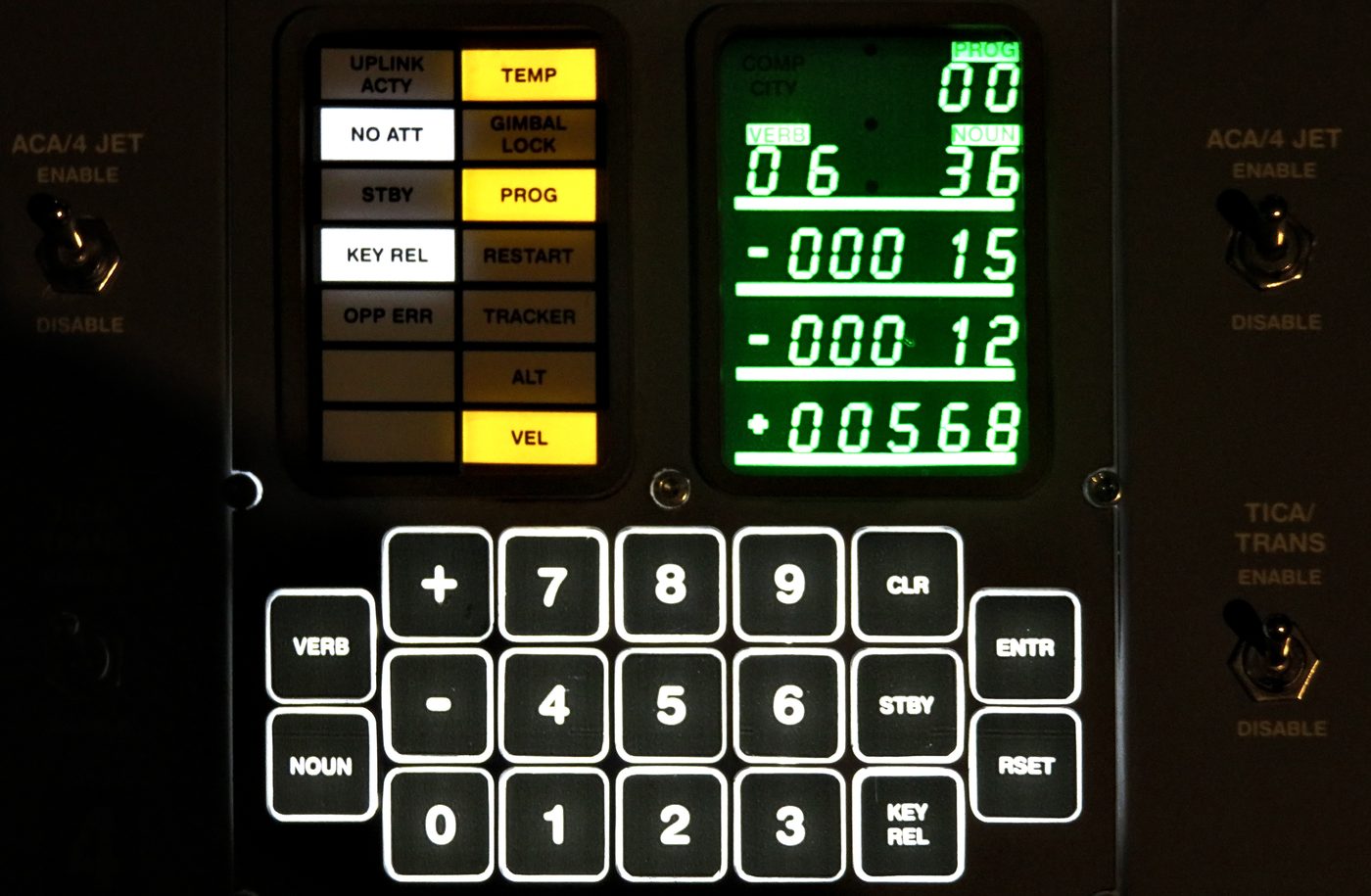
The second is the program interrupt: a true, vectored interruption that suspended the running program, saved just enough state, and transferred control to a fixed handler. A small number of interrupt lines existed, each with its own priority and its own dedicated entry point. The most important for the rhythm of the machine were the timed interrupts — periodic ticks (notably the TIME3/T3RUPT line tied to the waitlist and the executive’s scheduling cadence) that gave the software a regular heartbeat on which to hang scheduled tasks. Others served the DSKY keyboard, uplink, and downlink telemetry. When an interrupt fired, the handler ran, did its small urgent job, and executed a RESUME to restore the interrupted program exactly where it left off.

Together these formed the foundation of the AGC’s real-time executive. The counter interrupts maintained an always-correct sense of time; the timed program interrupts let the executive wake up on schedule, decide what most deserved the processor next, and dispatch it. Long computations could be interrupted and resumed without corruption; urgent ones could pre-empt the merely important. The famous 1201 and 1202 alarms of the Apollo 11 landing were this architecture working as designed under overload — the executive, swamped by spurious radar-driven work, shed low-priority tasks and restarted cleanly rather than freezing, precisely because the software had been built to fail gracefully on top of these interrupt and scheduling primitives.

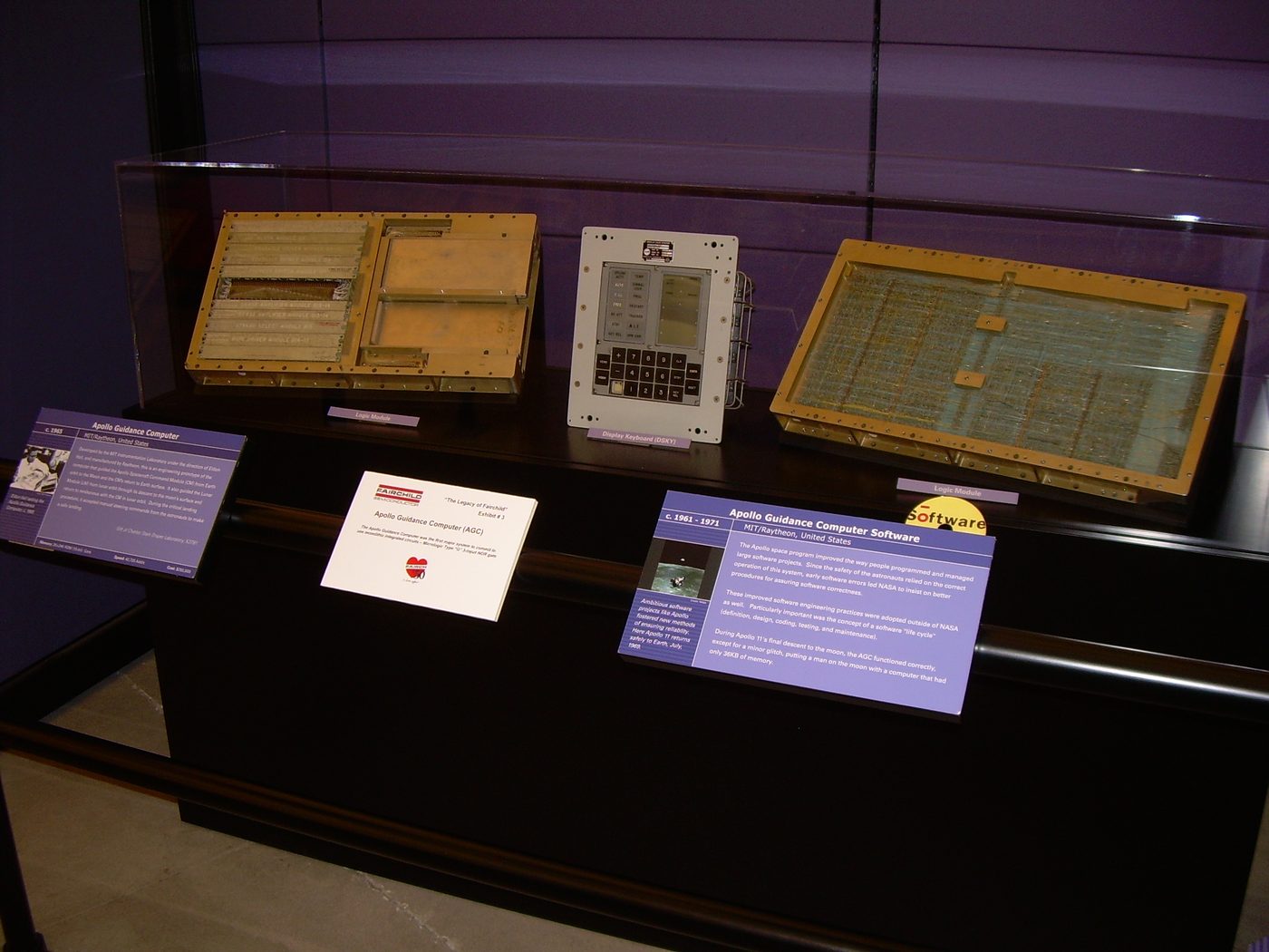
The Physical Machine

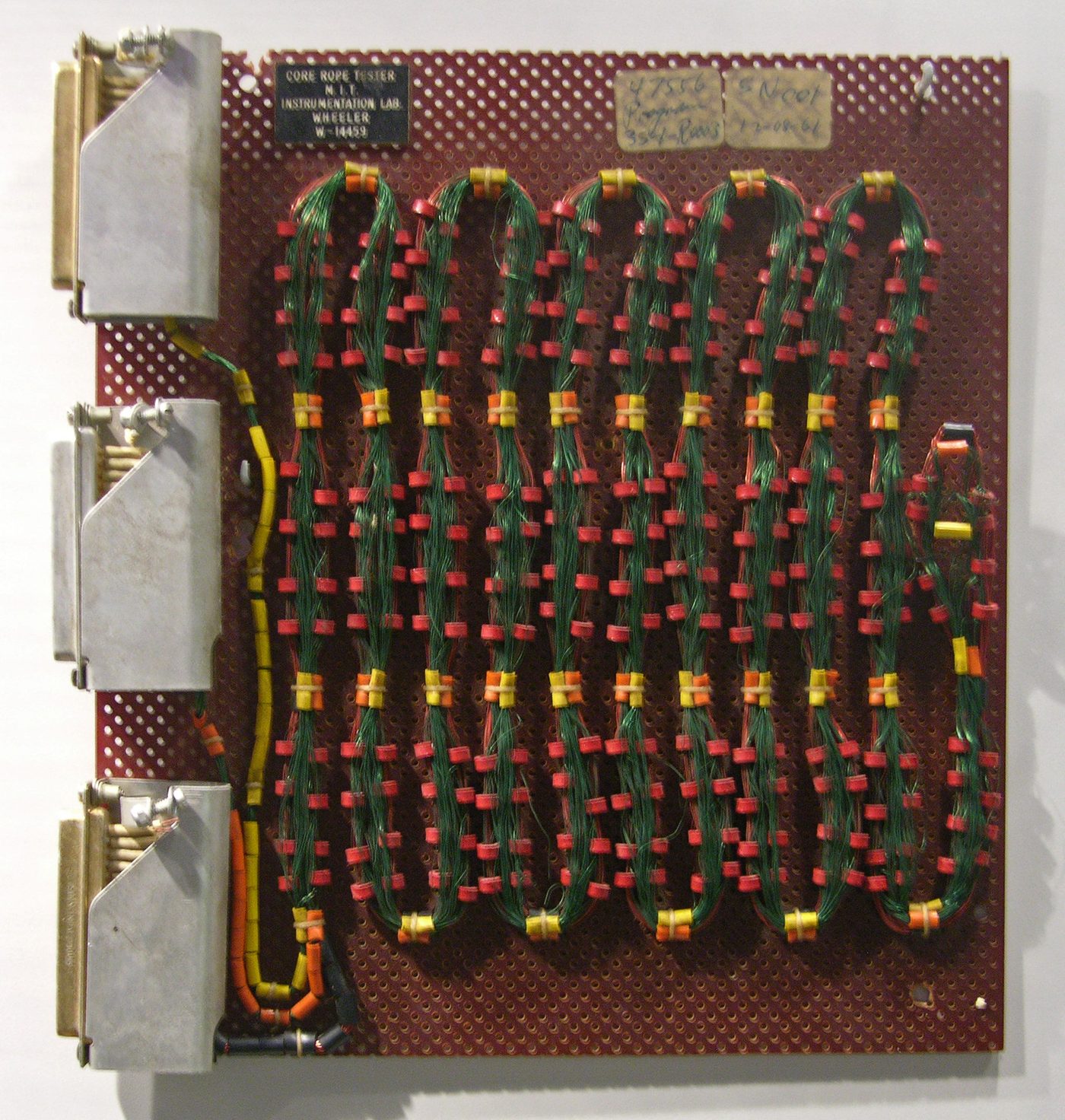
For all this logical sophistication, the AGC was a strikingly austere physical object: a sealed magnesium case, roughly the size of two stacked attaché cases, weighing about 70 pounds. Inside, the electronics were divided into two trays of pluggable modules. One tray held the logic — dozens of flat modules each carrying many of those identical dual-NOR-gate integrated circuits, potted and connected through the case’s woven backplane wiring. The other tray held memory and interface electronics: the erasable core memory, the read-only core rope modules that held the program, the oscillator, the power supplies, and the alarm and interface circuitry. Heavy multi-pin connectors at one end mated the computer to the spacecraft harness, the DSKY, and the inertial unit.

Every Apollo flight carried two of these machines, and they ran different software. One sat in the Command Module, running the program line known as Colossus; the other rode in the Lunar Module, running Luminary. They were the same architecture — same word, same registers, same instruction set, same interpreter — applied to two different vehicles and two different phases of the mission. That a single, small, fifteen-bit design could be trusted to fly men to the Moon and back, in two copies, is the clearest testament to how much careful thought was folded into its modest envelope.

We have now walked the machine from its smallest unit — a single fifteen-bit word with its lonely parity bit — up through clock, registers, instructions, interpreter, interrupts, and case. The next question is how this architecture came to be, because the Block II machine described here was the second AGC. The first was meaningfully different, and the journey between them is a story of hard-won lessons in reliability, manufacturability, and trust.

Next — Volume 7: Block I to Block II — Evolution of the Machine.